Sine and Cosine Functions

Sine

The function y=sin(x) is periodic with period 2 π and the value of y is limited to the range [-1 1]. Thus, an ANN can be used in mapping configuration to compute the value of y=sin(x).

Tip

The number of training cases is very important when training an ANN. Specifically, the number of training cases limits the number of neurons in the hidden layer. In some few problems, it is possible to modify the number of training cases; in other problems the number of cases in the data set is given and cannot be changed making impossible to increase the number of neurons in the hidden layer without producing overfitting.

Problem 1

Create a New Project called MappingSinCos using Neural Lab to build an appropriate training set to learn the functions: sin(x) and cos(x) as shown in the figure (we will use a General Purpose network application of a Multi-layer Network, you can save some typing by checking the Performace.lab checkbox in the project files). The training set will have 512 training cases using uniformly distributed values for x in the range from 0 to 2π.

Solution 1

Edit the BuildTrainSet.lab file and then

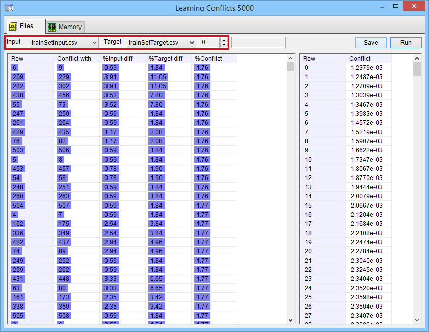
click the button to execute the code. If you do not have any errors, the training set will be generated and displayed on the variable list and the file list.

click the button to open the graph viewer and review the training set. Select the variables as shown.

MappingSinCos\BuildTrainSet.lab

int numCases = 512;
//_________________________________________ Build the input
Vector x;
x.CreateSeries(0.0, 2.0*3.1415926, numCases); // 0, ..., 6.28
Matrix trainSetInput;
trainSetInput = x;
//_________________________________________ Save the input
trainSetInput.Save();
//_________________________________________ Build the target
Vector sinx = sin(x);
Vector cosx = cos(x);
Matrix trainSetTarget = sinx;
trainSetTarget.AppendRight(cosx);
//_________________________________________ Save the target
trainSetTarget.Save();

Hint

An easy way to explore a data set is by making click on the data set file as follows:

Double click the file trainSetTarget.csv.
XY Plot click the button to plot the data.
See Columns click the button to plot each column.
Move the scrollbar at the right to review each column plot.

In this case, the first column (column 0) is a sine function and the second one (column 1) is a cosine function, see figure below.

Problem 2

Edit the BuildValidSet.lab file to build a validation set for the functions sin(x) and cos(x) using random values of x from 0 to 2π. Use 128 validation cases.

Solution 2

After editing the file,

click the button to execute the code. If you do not have any errors, the validation set will be generated and displayed on the variable list and the file list.

click the button to open the graph viewer and review the validation set. Select the variables as shown.

MappingSinCos\BuildValidSet.lab

int numCases = 128;
//_____________________________________________ Build the input
Vector x;
x.CreateRandom(numCases, 0.0, 2*3.1415926);
Matrix validSetInput;
validSetInput = x;
//_____________________________________________ Save the input
validSetInput.Save();
//_____________________________________________ Build the target
Vector sinx = sin(x);
Vector cosx = cos(x);
Matrix validSetTarget = sinx;
validSetTarget.AppendRight(cosx);
//_____________________________________________ Save the target
validSetTarget.Save();

Tip

Even though it is possible to use only one training method to train a network, it is also possible and more reliable to use a combination of two (or more) methods. The training must start with a non-greedy method such as: Simulated Annealing or Genetic Algorithm. Next, the training can be improved using: the conjugate gradient method (TrainConjGrad), the Levenberg Marquardt method (TrainLevenMar), or the variable metric method (TrainVarMetric) as shown in the figure. Any of the improving training methods take two parameters: the number of epochs and the desired goal.

Tip

The training process may include any training method. In most cases the training process is limited by time, computing resources or human patient. For instance the training described in the figure below begins by using simulated annealing, and then it continues using a genetic algorithm and ends with the conjugate gradient method.

Tip

The method of Levenberg Marquardt requires great amount of memory, and it can only be used when the network has very few outputs. For those applications that require a network with many outputs the method of conjugate gradient or variable metric should be used.

Tip

All the training methods have a set of parameters that need to be adjusted. Generally speaking, if the number of iterations or number or epochs increases, the running time increases. Always train an ANN using the maximum number of iterations as the time allows. A high number of iterations bring the possibility of a good training.

Problem 3

An ANN was trained using simulated annealing with 100 iterations per temperature. When the number of iterations was increased to 200, the training did not improve. What conclusions can be obtained from the experiment?

Problem 4

Use the Internet to find about the method of simulated annealing (cooling schedules, the metropolis algorithm, initial temperature, final temperature, etc.). Write a page about this method. You may include figures and graphs.

Problem 5

An ANN was trained using simulated annealing with 100 iterations per temperature and 10 temperatures. When the number of temperatures was increased to 50, the training improved considerably. What conclusions can be obtained from the experiment? What actions should be taken?

Problem 6

Use the Internet to find about genetic algorithms (initial population, probability of crossover, probability of mutations, etc.). Write a page about this method. You may include figures and graphs.

Problem 7

An ANN was trained using a genetic algorithm with 10 generations on a population size of 100. When the number of generations was increased to 50, the training improved considerably. What conclusions can be obtained from the experiment? What actions should be taken?

Problem 8

An ANN was trained using a genetic algorithm with 10 generations on a population size of 100. When the population size was increased to 200, the training improved insignificantly. What conclusions can be obtained from the experiment? What actions should be taken?

Problem 9

Use the Internet to find a typical value for the probability of mutation and the probability of crossover for genetic algorithms.

Problem 10

Edit the Train.lab file to design and train an ANN for the functions sin(x) and cos(x). Use one hidden layer and five neurons in this layer. As the number of outputs of this network is only one, the method of Levenberg Marquardt can be used. Train the ANN using simulated annealing, and the method of Levenberg Marquardt as shown:

Simulated Annealing:
Number of iterations = 100
Number of Temperatures = 100
Initial Temperature = 15
Final Temperature = 0.01
Cooling Schedule = Linear
Number of Cycles = 4
Goal (desired mse) = 1.0e-12

Levenberg Marquardt:
Number of Epochs = 1000
Goal (desired mse) = 1.0e-12

Solution 10

After editing the file,

click the button to execute the code. If you do not have any errors, the ANN will be trained when the code execution stops. Double click the network in the variable list to review the network. Then, select inputTrainSet.csv file and the targetTrainSet.csv file. You will be able to review the network behavior in real time by moving the scrollbar at the right. You can automatically generate the network code by using the Generate network code from the toolbar.

MappingSinCos\Train.lab

//_________________________ 1. Network Setup
LayerNet net;
net.Create(1, 5, 0, 2);
net.SetInScaler(0, 0.0, 2.0*3.1415927); // Input 0: values are from 0.0 to 6.2833
net.SetOutScaler(0, -1.0, 1.0); // Output 0: values are from -1.0 to 1.0
net.SetOutScaler(1, -1.0, 1.0); // Output 1: values are from -1.0 to 1.0
//________________________ Load and set the training set
Matrix trainSetInput;
trainSetInput.Load();
Matrix trainSetTarget;
trainSetTarget.Load();
net.SetTrainSet(trainSetInput, trainSetTarget, false);
//________________________ 2. Train using Simulated Annealing
net.TrainSimAnneal(
     20, //Number of Temperatures
     20, //Number Iterations
     15, //Initial Temperature
     0.001, //Final Temperature
     true, // Is Cooling Schedule Linear?
     1, // Number of Cycles
     1.0e-5 // Goal (desired mse)
);
//________________________ 3. Train using Genetic Algorithms
//net.TrainGenetic(
//     100, // Population Size
//     20, //Number Generations
//     1.5, // Over Population
//     0.001, // Probability of Mutation
//     0.8, // Probability of Crossover
//     1.0e-12); // Goal (desired mse)
//________________________ 4. Train using Levenberg Marquardt
//net.TrainLevenMar(1000,1.0e-10); // Epochs and Goal
net.TrainConjGrad(1000, 1.0e-10);
//________________________ 5. Save the trained network
net.Save();

Tip

When looking at the network simulation, some of the output values are displayed in red. The red color indicates that the actual output network and the desired target are not equal for the current training case. You may use the scrollbar on the right side to review and analyze other training cases. When the network and the training are properly performed, the red color should appear in only very few cases or should not appear at all.

Problem 11

Double click the network in the variable list of the last problem to see the network. Then, select inputTrainSet.csv file and the targetTrainSet.csv file.

click the tab to see the error by each training case.

click the button to see the error for each output. What conclusions can be reached from these graphs?

Problem 12

In the network of problem 10, modify the number of hidden neurons to 10. Train the network and compute the error for each training case. What conclusions can be reached by comparing the error when the network had 5 neurons in the hidden layer?

Problem 13

In the network of problem 10, modify the number of hidden neurons to 20. Train the network and compute the error for each training case. What conclusions can be reached by comparing the error when the network had 5 and 10 neurons in the hidden layer?

Problem 14

Using the network trained in the last problem, double click the network to perform a simulation in real time use validSetInput.csv instead of trainSetInput.csv, and validSetTarget.csv instead of trainSetTarget.csv to perform the simulation. Is the behavior of the ANN different when the number of neurons in the hidden layer is modified?

Problem 15

Edit and run the CheckTraining.lab file to check the training: (a) Compute the mean squared error for the ANN (20 neurons in the hidden layer) using the training set. (b) Plot the error for each training case. (c) Save the plot as a vector image (checkTraining.emf and checkTraining.pdf)

Problem 16

Edit and run the Validation.lab file to perform the validation of the ANN. (a) Compute the mean squared error for the ANN (20 neurons in the hidden layer) using the validation set. (b) Plot the error for each validation case. (c) Save the plot as a vector image (validation.emf and validation.pdf)

Problem 17

Write some code to graph the mse for the validation and for training as a function of the number neurons in the hidden layer from 0 to 19. This test may last several hours.

Solution 17

click the button to create a new code file called PerformanceTest. Write the code show below.

click the button to execute the code. You will be asked to save the file, set the file name to PerformanceTest.lab. If you do not have any errors, the mse for both training and validation will be displayed in the variable list.

click the button to open the Graph Viewer and select the variables as shown. Be sure to use a logarithmic scale on the Y-axis. What conclusions can be obtained from the graphs?

MappingSinCos\PerformanceTest.lab

//________________________ Load and set the training set
Matrix trainSetInput;
trainSetInput.Load();
Matrix trainSetTarget;
trainSetTarget.Load();
//_______________________ Load the validation set
Matrix validSetInput;
validSetInput.Load();
Matrix validSetTarget;
validSetTarget.Load();
//________________________ Network setup
int numHidden = 1;
LayerNet net;
Matrix output;

Vector mseTraining;
mseTraining.Create(20);

Vector mseValidation;
mseValidation.Create(20);

for(numHidden = 0; numHidden < 20; numHidden++)
{
     net.Create(1, numHidden, 0, 2);
     net.SetInScaler(0, 0.0, 2.0*3.151927);
     net.SetOutScaler(0, -1.0, 1.0);
     net.SetOutScaler(1, -1.0, 1.0);
     net.SetTrainSet(trainSetInput, trainSetTarget, false);
     //
     net.TrainSimAnneal(100, 100, 15, 0.01, false, 4, 1.0e-12);
     //net.TrainGenetic(100, 100, 1.5, 0.01, 0.7, 1.0e-12);
     //net.TrainLevenMar(1000,1.0e-12);
     //_____________________________________________ check training
     output = net.Run(trainSetInput);
     mseTraining[numHidden] = ComputeMse(output, trainSetTarget);
     //_____________________________________________ validation
     output = net.Run(validSetInput);
     mseValidation[numHidden] = ComputeMse(output, validSetTarget);
}
mseTraining.Save();
mseValidation.Save();

Problem 18

Choose an appropriate number of neurons in the hidden layer and train the network. Write the file TrainSim.lab to compare the actual output of the network and the target using the training set.

MappingSinCos\TrainSim.lab

LayerNet net;
net.Load();
//_____________________________________ Input
Matrix trainSetInput;
trainSetInput.Load();
//_____________________________________ Target
Matrix trainSetTarget;
trainSetTarget.Load();
Vector sinTarget = trainSetTarget.GetColVec(0);
Vector cosTarget = trainSetTarget.GetColVec(1);
//_____________________________________ ANN output
Matrix output = net.Run(trainSetInput);
Vector sinNN = output.GetColVec(0);
Vector cosNN = output.GetColVec(1);

Problem 19

From Neural Lab toolbar click on Learning Conflicts to analyze the training set. The figure below shows the learning conflicts in the first column in the training set. You can optionally, compute the learning conflicts in the second column in the training set. The Learning Conflicts tool allows you to find errors in your datasets.

Problem 20

Choose an appropriate number of neurons in the hidden layer and train the network. Write the file ValidSim.lab to compare the actual output of the network and the target using the validation set. As the validation set has random input points, we cannot use the original validation set. Instead we use a uniformly distributed validation set as shown (note that the number of points cannot be the same as the training set; in fact the number of points must be chosen carefully so that the cases in the validation set are the same as those in the training set).

MappingSinCos\ValidSim.lab

LayerNet net;
net.Load();

int numCases = 300;
//_____________________________________________ Build the input
Vector x;
x.CreateSeries(0.0, 2.0*3.1415926, numCases); // 0, ..., 6.28
//_____________________________________ Target
Vector sinx = sin(x);
Vector cosx = cos(x);
//_____________________________________ ANN output
Matrix output = net.Run(x);
Vector sinNN = output.GetColVec(0);
Vector cosNN = output.GetColVec(1);

Problem 21

Create an independent application for Microsoft Windows using C++ to compute the sine and cosine of a value using an ANN.

Solution 21

For this problem you will require Microsoft Visual Studio and Wintempla. Links to download Microsoft Visual Studio and Wintempla are found in the main page of this tutorial (Academic Software

Install Microsoft Visual Studio, if you have not done so
Install Wintempla, if you have not done so
Open Microsoft Visual Studio > File > New > Project > Visual C++ > Wintempla > Dialog Application (Set the name to Calculator and set an appropriate location to create the project)
From Microsoft Visual Studio open Wintempla Tools>Wintempla
Draw five labels, five text boxes and one button as shown. Be sure to assign the names as shown in the figure.
Edit the file Calculator.h as shown below (write only what it is marked in red)
Edit the file Calculator.cpp as shown below (write only what it is marked in red)
Run the program Debug > Start debugging (if you have no errors, the calculator will open)

Be sure the program can locate the net.lay file. Microsoft Visual Studio will try to open this file at the Calculator\Calculator folder. You need to copy the net.lay file from its original location to Calculator\Calculator\net.lay.

Problem 22

Generate a report in Microsoft Word. Write some conclusions in the report focusing on the problems that were faced during the simulation and how these problems were or could be solved.

Sine and Cosine Functions

Sine

© Copyright 2000-2021 Wintempla selo. All Rights Reserved. Jul 22 2021. Home